Beginner
Introduction to H2O Hydrogen Torch: Coins sum
This tutorial uses H2O Hydrogen Torch to train an image regression model that predicts the sum of Brazilian Real (R$) coins in images. This model is expected to work on new coins of the same currency. While training this model, we will see how H2O Hydrogen Torch enables you to generate accurate models with expertly default hyperparameter values that H2O Hydrogen Torch derives from model training best practices used by expert data scientists and top Kaggle grandmasters.
Also, we will discover how H2O Hydrogen Torch enables you to monitor and understand the impact of selected hyperparameter values on the training process through simple interactive charts.
Completing this tutorial should improve your understanding of H2O Hydrogen Torch.
Prerequisites
- Basic knowledge about neural network training
Step 1: Explore dataset
For this tutorial, we will be using the preprocessed Coins Default Image Regression dataset that comes preloaded in H2O Hydrogen Torch. The dataset contains a collection of 6,028 images with one or more coins. Each image has been labeled to indicate the sum of its coins. The currency of the coins is the Brazilian Real (R$).
Note
The Coins Default Image Regression dataset was preloaded using the S3 connector. To learn more, see Data Connectors.
As a requirement, H2O Hydrogen Torch requires the dataset for an experiment to be preprocessed to follow a certain dataset format for the problem type the experiment aims to solve. The Coins Default Image Regression dataset was preprocessed to follow a dataset format for an image regression model.
Note
-
To learn about the dataset format for an image regression experiment and about the format of the Coins Default Image Regression dataset, see Image Regression.
-
To learn about the format a dataset needs to follow under a particular supported problem type, see Dataset Formats.
On the View datasets card, you can locate all imported datasets in H2O Hydrogen Torch. With that in mind, let's explore the Coins Default Image Regression dataset.
-
In the H2O Hydrogen Torch navigation menu, click View datasets.
-
In the View datasets card, click coins_default_image_regression.
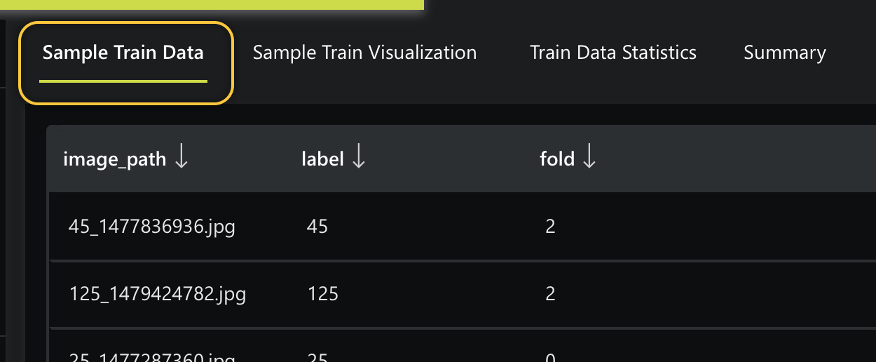
On the Sample Train Data tab, we can observe 3 columns and few of the 6,028 rows in the Coins Default Image Regression dataset. Each row in the dataset contains a name of an image (image_path) depicting several coins that add up to a certain sum recorded in the label column:
Note
-
During model training, the
foldcolumn splits the data into subsets. A separate model is trained for each value in thefoldcolumn where records with the corresponding value form a holdout validation sample while all the remaining records are used for training. A holdout validation sample is created if a validation dataframe is not provided during an experiment. Five-folds are assigned randomly for any experiment where the dataset does not contain afoldcolumn, which is sometimes not the desired strategy. The fold column can include integers (0, 1, 2, … , N-1 values or 1, 2, 3… , N values) or categorical values. -
For this regression model, we are not using a validation dataframe.
To view a few visual examples of the dataset rows, click the Sample Train Visualization tab. If you hover over one of the images, the label (sum) of the image appears:
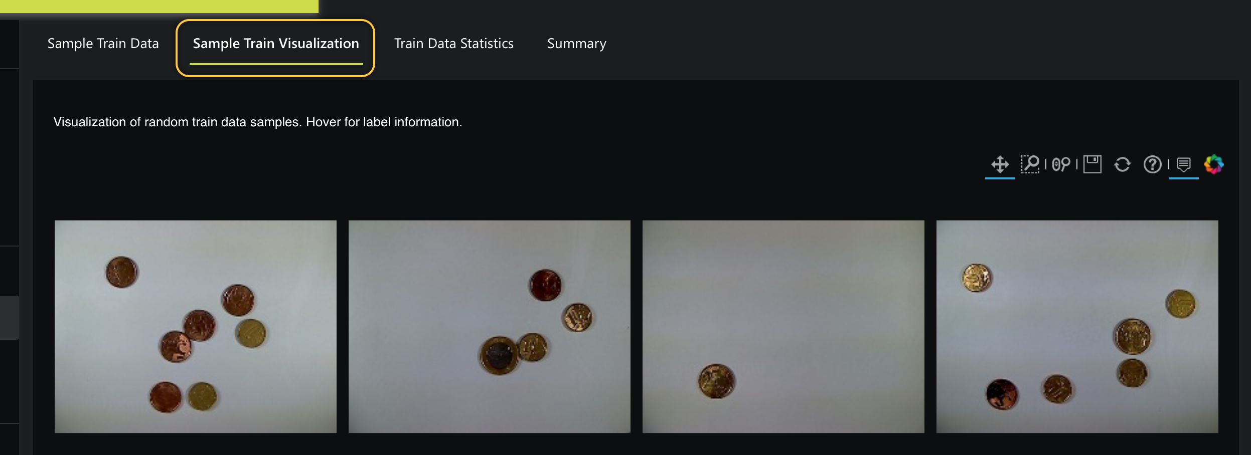
Now that we better understand the Coins Default Image Regression dataset let's build a model that will predict the sum of coins an image contains.
Step 2: Run experiment
-
In the H2O Hydrogen Torch navigation menu, click Create experiment.
Several experiment settings are available on the Create experiment card; by default, every time you access the Create experiment card, H2O Hydrogen Torch will present you with settings for the problem type the oldest imported dataset aims to solve.
-
Scenario 1: If you haven't imported any other datasets, the Create experiment card will provide settings for an Image Regression experiment. In particular, the default experiment settings (hyperparameters) will be for the Coins Default Image Regression dataset.
-
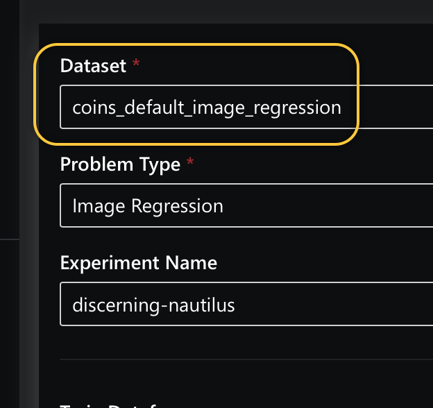
Scenario 2: If you have imported other datasets, proceed with the following instructions to ensure that the Coins Default Image Regression dataset is selected. Selecting this dataset will display default settings for a regression model:
a. On the Create experiment card: In the Dataset box, select coins_default_image_regression.
For all the settings available for an image regression model, H2O Hydrogen Torch has defined each setting with a default value while considering model training best practices used by top Kaggle grandmasters.
Note
-
All the settings available for all problem types in H2O Hydrogen Torch have been provided with a default value while considering model training best practices used by top Kaggle grandmasters.
-
To learn about the available settings for an image regression experiment, see Experiment settings: Image regression.
Before we continue, note that models are evaluated using a model scorer, and for our model, the default scorer is the Mean Absolute Error (MAE). For our model purposes, we want a validation score value of 0 for our experiment, indicating an excellent prediction value where all predictions' loss value is 0. Loss refers to the penalty for a bad prediction.
The closer the MAE value (validation score) approximates to 0, the better (in regards to each prediction having a lower loss value).
The validation score will represent, on average, how much the model predictions (sums) are off compared to the true sums. Accordingly, the model being off will also refer to loss, which will indicate the loss is greater than zero.
Note
Loss indicates how bad the model's prediction was on a single example. A loss value of zero for a given single example will indicate that the model's prediction is perfect.
-
-
With the above in mind, click Run experiment.
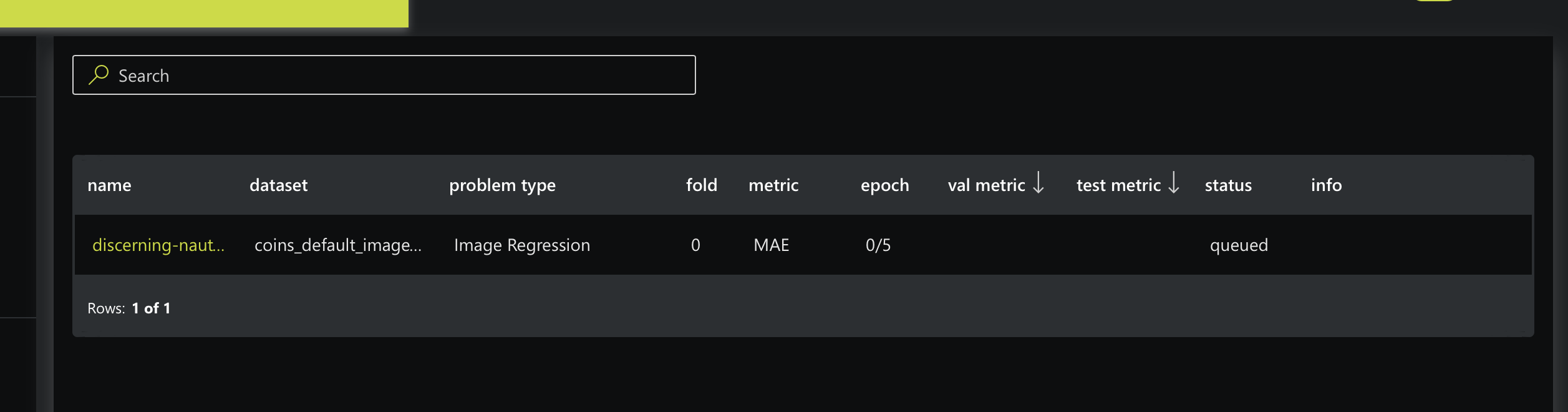
After starting your experiment, H2O Hydrogen Torch will take you to the View experiments card, where you can view running and completed experiments:
Step 3: Observe Running Experiment
As the experiment completes, let's observe the performance of our image regression model through simple and interactive charts.
The prediction metrics from your experiment might differ from those discussed from this point on.
-
On the View experiments table, click discerning-nautilus (random name H2O Hydrogen Torch assigned to our experiment). In your case, pick the name of your experiment. The following charts appear (on the Charts tab):
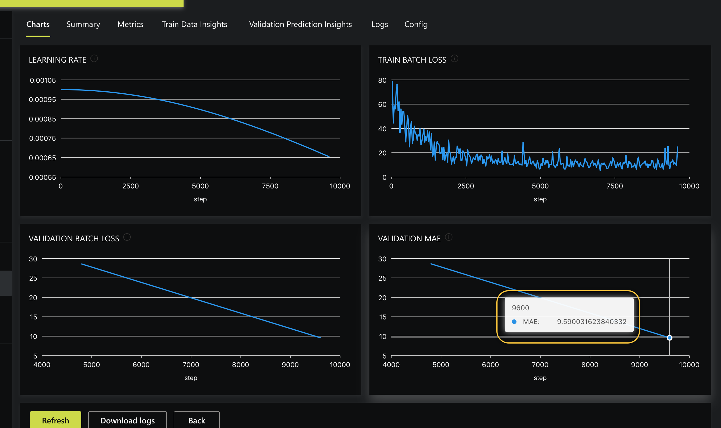
Hovering over the Validation MAE chart, we see that after the second Epoch is completed, the MAE decreases to 9.590.
Note
Recall, the closer the MAE value (validation score) approximates to 0, the better.
As the experiment completes each Epoch, the charts on the Charts tab will be updated until H2O Hydrogen Torch completes the experiment. To visualize the impact of this MAE decrease, let's see what the Validation Prediction Insights tab contains.
-
Click the Validation Prediction Insights tab. The following prediction metrics appear:
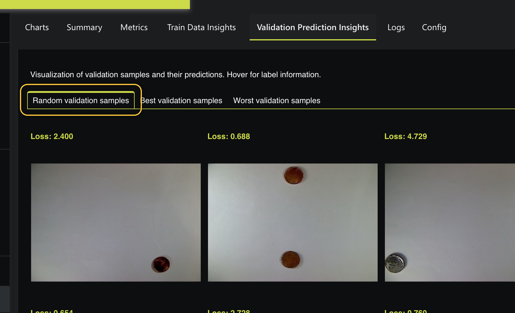
In this case, on the Random validation samples tab, we can see random validation samples highlighting the best, and worst validation samples as each Epoch is complete. Viewing several validation samples can tell us how the experiment is doing in terms of achieving a low (good) validation score. Hovering on one of the random validation samples, we can see the predicted and actual sum of the image. As well, each validation sample contains a Loss value.
Note
- The examples on the Validation Prediction Insights tab come from a created validation dataset. During training, if a validation dataset is not provided, H2O Hydrogen Torch holds back a few samples from the training dataset to create a validation dataset used to validate the training loss. Recall that we did not provide a validation dataset.
Now, let's wait until the experiment is complete.
Step 4: Observe Completed Experiment
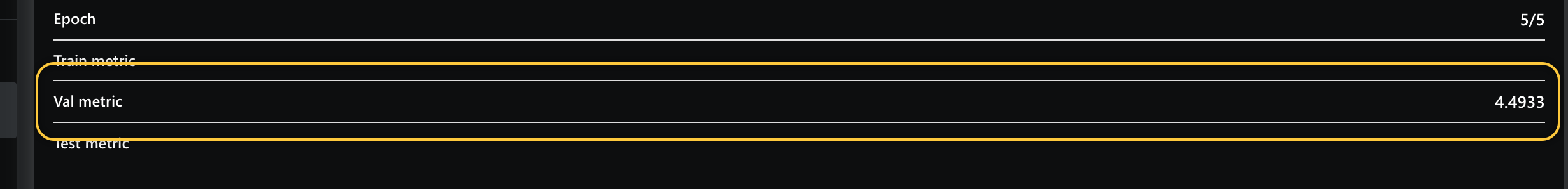
Now that our experiment is complete, let's observe the validation score (Val metric). According to the summary tab, the final validation metric is 4.4933 (by how much the model is off):
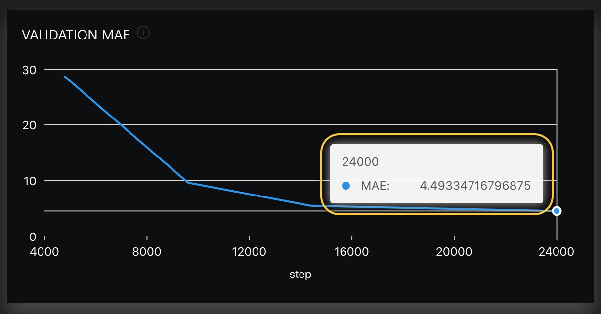
You can also view the final validation score in the Validation MAE chart (on the Charts tab) that highlights the Validation MAE across time while each epoch was completed:
At this point, we might be wondering when will it be good or bad to implement this built model in production:
-
Use Case 1: Suppose an Automated teller machine (ATM) accepts coins as a deposit while using our built model. In this scenario, our built model's validation MAE can be viewed as low-performing, leading to someone's coins deposit being over or undercounted. Not suitable for the bank ATM if the model overcounts and good for the customer if it does. The model will not be acceptable under this use case because an ATM is expected to count accurately. With that in mind, we will need to tune the hyperparameters to improve the validation MAE.
-
Use Case 2: Suppose you want to obtain a rapid approximate sum of many coins using our built model. In this scenario, we first need to define an acceptable margin of error for a rapid approximation. If our built model's validation MAE can match the defined acceptable margin of error, we can say the model in this scenario will be acceptable (well-performing).
Note
A well-performing model will be defined by an acceptable solution within the constraints and expectations of the use case.
To further understand the final validation score, we can reexplore the Validation Prediction Insights tab to learn from all the best and worst validation samples now that the experiment is complete. In particular, we can explore the type of images the model was good or bad at predicting.
-
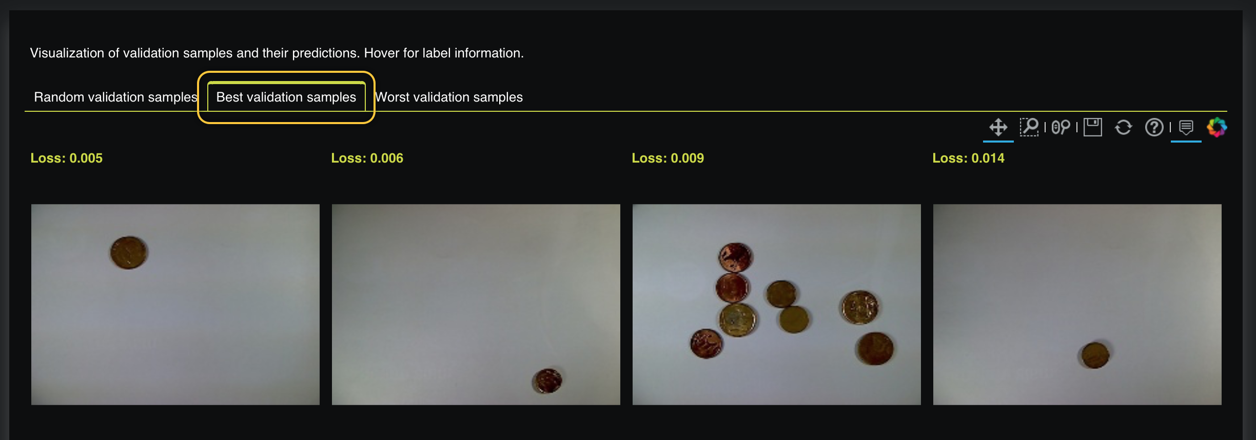
On the Validation Prediction Insights tab, click Best validation samples. Here, we can see the best validation samples where a prediction's loss value is low when compared to other samples:
-
On the Validation Prediction Insights tab, click Worst validation samples. Here, we can see the worst validation samples where a prediction's loss value is high when compared to other samples:
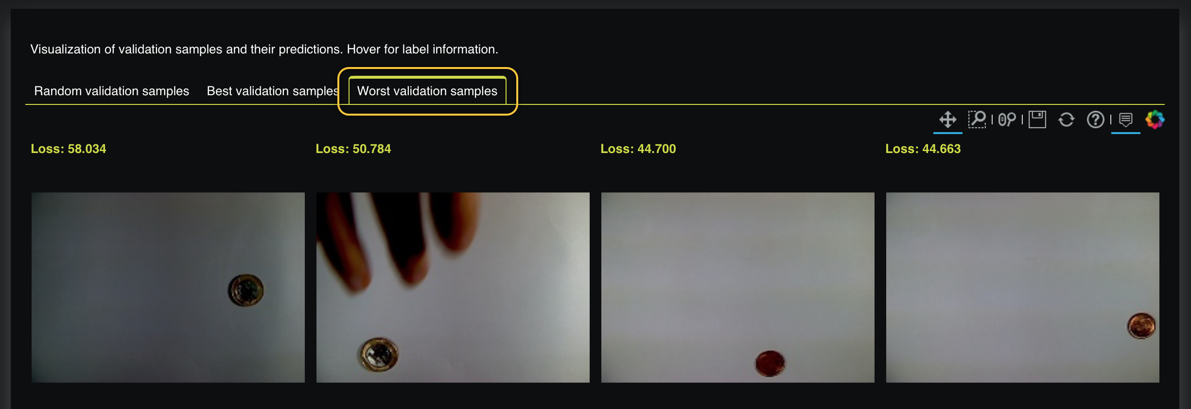
Observing the best and worst validation samples shows that high loss values were generated anytime the image was too dark. With this in mind, we can assume that replacing these dark images with more clear ones can lead to a better validation score because clear images will allow our regression model to learn from clear images where coins can be distinguished.
Summary
In this tutorial, we learned the basic workflow of H2O Hydrogen Torch. In particular, we learned that H2O Hydrogen Torch enables data scientists to modify an array of hyperparameters that potentially can improve training performance and predictions.
We discovered that H2O Hydrogen Torch provides several interactive graphs and easy-to-understand visuals to monitor and understand performance metrics and predictions during and after an experiment. The knowledge you have gained from this beginner tutorial should give you the confidence to use H2O Hydrogen Torch to experiment quickly on hyperparameters for different problem types, resulting in world-class models that accurately predict your target of choice.
Once you have trained your model, you can deploy the model into production. To learn more, see Deployment Options.
- Submit and view feedback for this page
- Send feedback about H2O Hydrogen Torch to cloud-feedback@h2o.ai